The Excel Add-In is an alternative way to enter, update, manage, query and analyze application data, using Excel spreadsheets and workbooks.
You can use the Excel Add-In to:
-
Query and submit data into the application.
-
Change the cube point of view.
-
Interact with forms.
-
Leverage multiple cube views.
-
Establish a live connection to cube views in the application.
-
Drill through to source data.
-
Create functions to return, amend, or submit application data.
-
Refresh sheets and workbooks when changes occur in the application.
You can launch Excel documents from:
-
The Navigation pane
-
The OnePlace tab: Through public and user-specific access to application functionality and documents.
-
The Application tab: Through the Spreadsheet tool.
-
The System tab: Using export features for system administrators.
-
-
Workflow forms that have attached templates.
-
Cell or data unit attachments.
-
Dashboards
-
Cube views
-
File Explorer
Excel Add-In
Before you start using Excel Add-In, you must add the OneStream ribbon to your Excel program.
Add the OneStream Ribbon
-
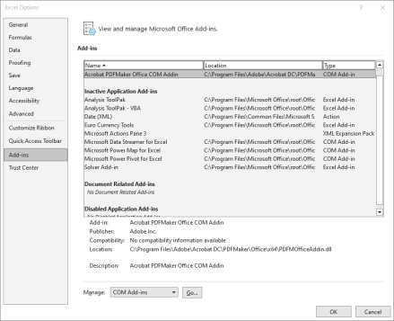
In an Excel workbook, navigate to File > Options to open the Excel Options dialog.
-
Select Add-ins from the menu in the left pane. Click the Manage drop down menu at the bottom of the dialog box and select COM Add-ins and then click Go.
-
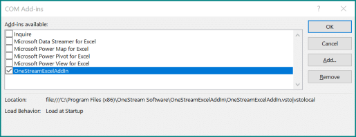
Click the box next to OneStreamExcelAddIn and then click OK.
-
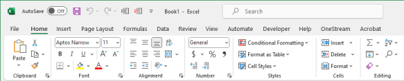
The OneStream ribbon is displayed at the top of your workbook page.
Log Into the Excel Add-In
-
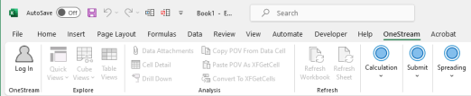
From the OneStream ribbon in Excel, click Log In.
-
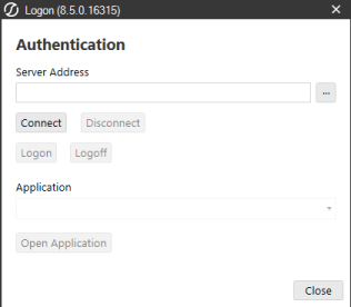
In the Server Address field, click the ellipsis to add or select the URL for the server.
-
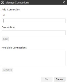
Select an available connection or add a new connection by entering the URL and description and clicking Add. After you select a connection, click OK.
-
Click Connect to authenticate the server.
-
Enter your username and password and click Logon.
-
In the application field, select an application and click Open Application.
After completing the authentication files and opening the application, your username and application name display in your Excel workbook, indicating that you are logged into the Excel Add-In.

Update the Excel Add-In
If you use the Excel Add-In provided with the Windows application, update the Excel Add-In as part of your client update. See Client Updater. Otherwise, update the Excel Add-In by uninstalling then reinstalling it as described in the Installation Guide.
Compatibility
OneStream makes every effort to support complex environments and maintain compatibility with other add-ins, by testing our Excel Add-in using a standard desktop deployment. There are factors outside our control which can negatively impact compatibility, so we cannot make a guarantee or warranty of service for compatibility.
Excel Add-In
Excel Add-In › Add-In Components
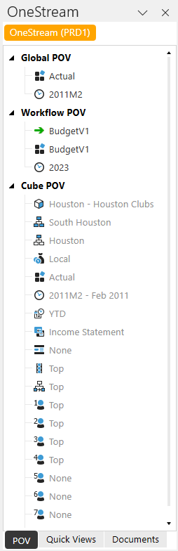
The Excel Add-in Task pane includes the POV, Quick Views and Documents tabs as shown below.
-
POV: Identifies the Global POV, Workflow POV, and Cube POV. This tab is linked to the POV in your application. From here, you can make updates to the cube POV.
-
Quick Views: Lets you build and edit quick views in the Excel Add-in. See Quick Views.
-
Documents: Displays public or user-specific application or system documents. Access and manage documents with the File Explorer.
Excel Add-In › Add-In Components
After installing the Excel Add-In, there will be a OneStream menu item and a ribbon in Excel. The ribbon contains these categories:
NOTE: When working in Excel, decimals are automatically truncated after the ninth character in a cell or a function.
OneStream
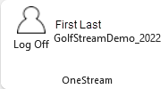
This displays the current user and application. A user can log off or logon to a different application by clicking this icon.
Explore
The Explore category enables you to quickly build a Quick View, Cube View, or Table View in Spreadsheet or Excel.
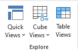
Quick Views
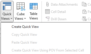
Create Quick View
This will create a new Quick View in the worksheet’s selected cell.
Copy Selected Quick View
This will copy the selected Quick View in order to paste a version of it in another spreadsheet or workbook.
Paste Quick View
This will paste the copied quick view to the current spreadsheet or another workbook.
Create Quick View Using POV from Selected Cell
This will create a new Quick View based on the current POV from the selected cell. This can be done using a Quick View cell’s POV or a Cube View cell’s POV.
See Quick Views for more information.
Cube Views
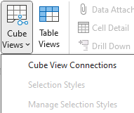
Cube View Connections
Create a new Cube View Connection in the selected cell. .
Selection Styles
Create selection styles for Cube Views. See Selection Styles for Cube Views.
Manage Selection Styles
This enables you to modify available selection styles.
Table Views

Select Table Views to insert a Table View into your Excel sheet.
Analysis
Data Attachments
This pulls up the Data Attachments dialog to show existing comments or attachments on a selected cell, or to allow data attachment edits.
Cell Detail
Enter Cell Detail for a Cube View or Quick View data cell.
Drill Down
Drill down on a specific cell in order to see more details or gather more information.
Copy POV from Data Cell
This captures the Point Of View of the currently selected cell. After clicking this option, the Paste POV As XFGetCell becomes available and the Copy POV From Data Cell goes to gray. The ability to paste this into another cell is now available and OneStream will automatically convert this into an XFGetCell formula with all of the appropriate Parameters.
Paste POV As XFGetCell
This option is only available after clicking Copy POV From Data Cell. After clicking this option, OneStream will convert the copied cell into an XFGetCell formula. Click Refresh Data to retrieve the data.
Convert to XFGetCells
This will convert an existing Quick View into an XFGetCells. After clicking this option, OneStream will prompt with the following: Are you sure you want to convert all of the data in Quick View ‘Name of the Quick View’ to XFGetCells? By clicking OK, the Quick View definition will be deleted and converted to XFGetCells.
Refresh
Refresh Sheet
This pulls down updated data from the server and only refreshes the selected worksheet.
Refresh Workbook
This pulls down updated data from the server and refreshes the entire Excel workbook.
| Refresh Sheet | Refresh Workbook | |
|---|---|---|
| Function Behavior | Refreshes the selected tab only | Refreshes all tabs in the file |
| Data Impacts | Clears all dirty cells on the selected tab only | Clears all dirty cells on all tabs regardless of selected tab |
| Parameter Impacts (CV Only) | Prompts the user with any Parameters used on the selected tab | Prompts the user with all the Parameters used in the workbook |
Calculation
Consolidate/Translate/Calculate
If permission is granted, these calculations can be performed on the selected cell.
Submit
Submit Sheet
After editing data in Excel, click this icon to send it back to OneStream for Cube Views, Quick Views, XFSetCells, and Table Views on the active sheet.
Submit Workbook
After editing data in Excel, click this icon to send it back to OneStream. This icon will send data back for every tab in the Excel workbook.
| Submit Sheet | Submit Workbook | |
|---|---|---|
| Function Behavior | Identifies data changes on the selected table and stores these changes to the database | Identifies data changes on every tab and stores these changes to the database |
| Data Impacts | Submits all data for the selected tab only | Submits all data for all tabs |
| Parameter Impacts (CV Only) | No prompts | No prompts |
Spreading
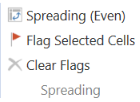
Enables users to see what type of spreading was used to spread data values over several columns or rows without having to type in each cell’s values.
Spreading Types
Fill
This fills each selected data cell with the value in the Amount to Spread property.
Clear Data
This clears all data within the selected cells.
Factor
Multiply all cells by the specified rate.
Accumulate
This takes the first selected cell’s value and multiplies it by the rate specified. It then takes that value, multiplies it by the specified rate and places it in the second cell selected, and does this for all selected cells. For example, four cells are selected and the first cell has a value of 900.
Even Distribution
This takes the Amount to Spread and distributes it evenly across the selected cells.
445 Distribution
This takes the Amount to Spread and distributes it with a weight of 4 to the first two selected cells and a weight of 5 to the third cell.
454 Distribution
This takes the Amount to Spread and distributes it with a weight of 4 to the first selected cell, a weight of 5 to the second cell and a weight of 4 to the third.
544 Distribution
This takes the Amount to Spread and distributes it with a weight of 5 to the first selected cell and a weight of 4 to the second and third cells.
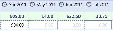
The Accumulate Spreading is setup as follows with a rate of 1.5:
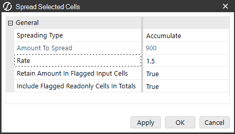
When the spreading is applied the outcome is as follows:
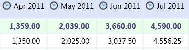
Each cell’s value is a factor of the previous cell amount.
Proportional Distribution
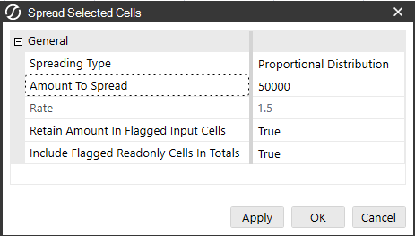
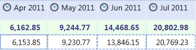
This takes the selected cell’s value, multiplies it by the specified Amount to Spread, and then divides it by the total sum of all selected cells. If all the cells have a zero value, the Amount to Spread will behave like an Even Distribution.
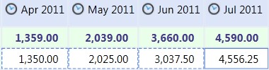
A proportional amount of 50,000 is applied to the cells:
Result:
Spreading Properties
Amount to Spread
Specify the value to spread over the selected cells. The value defaults to the last cell selected. The way the amount in this field spreads varies by Spreading Type.
Rate (Factor and Accumulate Spreading Types Only) Enter a rate to multiply by a cell value.
Retain Amount in Flagged Input Cells
Users can flag specific cells in order to retain the data within the cell. If this property is set to True, spreading will not apply to the selected flagged cells.
Include Flagged Readonly Cells in Totals
Set this to True to include locked base-level cell values when calculating spreading totals. True is the default.
Flag Selected Cells
Flags selected cells so the original amount in the cell is retained during the spreading process.
Clear Flags
Select this to clear any flagged cells.
File Operations
File Explorer
Use File Explorer to upload and download files.
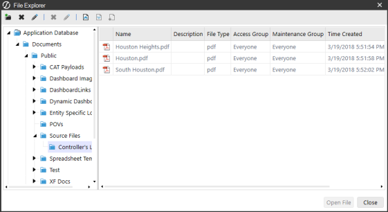
 Create Folder
This creates a new folder under the selected folder on the left-hand side of the File Explorer pane.
 Delete Selected Folder/File
This deletes the selected folder on the left-hand side of the File Explorer pane or the selected file.
 Edit Selected Folder/Edit Selected File Information
This edits the Description, Maintenance Group, and Access Group for the selected folder or file.
 Upload File
This uploads the selected file and allows the user to save.
 Download Selected File
This downloads the selected file and allows the user to save.
 Download Selected File’s Content File
This downloads the selected file’s content file and allows the user to save.
Save to Server
Use this option to save your file to the OneStream folder structure. You can save files to any location matching your security access. If the file was opened from a OneStream location, it will be saved back to that location. If it wasn't, File Explorer will open.
Save Offline Copy
Use this to save an offline copy of the current worksheet without the functions. Users without the Excel Add-In can open this copy and see the saved values.
General
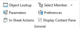
Object Lookup
Use the Object Lookup to insert objects from OneStream into Excel such as Foreign Exchange Rate Types when building formulas. If creating an Extensible Document in Excel, users can use the Object Lookup to insert Parameters, Substitution Variables, or Image Content. See Object Lookup in Presenting Data With Books, Cube Views and Dashboards for more details on this feature.
In-Sheet Actions
Create buttons to execute a Data Management Sequence, Submit data, or Refresh data, without leaving the sheet. See In-Sheet Actions.
Parameters
Insert a new parameter to quickly filter Cube Views and Table Views or manage existing parameters in the workbook. See Parameters.
Select Member
Select a Dimension Type from the drop-down list in order to view the Members of that Dimension. Select a Member of the hierarchy, and the Member name will display in the selected cell.
Preferences
Set Preferences for how to interact with and display your OneStream data. Settings include:
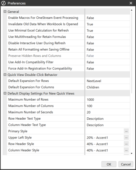
General
-
Enable Macros for OneStream Event Processing: If set to True, this enables Excel macros for OneStream API calls. The default is False.
-
Invalidate Old Data When Workbook is Opened: If set to True, this will force a data refresh on the opened workbook. The default is False.
-
Use Minimal Calculation for Refresh: This is for Excel Add-In only, not the Spreadsheet feature in OneStream Windows App. The default is True this will only calculate formulas and Excel functions in the active sheet. Set to False to revert to a full calculation of all workbooks and all sheets.
NOTE: Performance is best when Excel is set to use Manual Calculation Mode.
-
Use Multithreading for Retain Formulas: When set to True, processing steps for collecting and applying formulas to Cube Views with retain formulas enabled will run concurrently for multiple worksheets, allowing for faster refresh rates. This is for Excel Add-In only, not the Spreadsheet feature in OneStream Windows App.
-
Disable Interactive User During Refresh: Accounts for a known Excel situation when running on certain touchscreen hardware. If the Refresh Sheet or Refresh Workbook is pressed but the cells containing functions do not complete their calculations when processed, change the Disable Interactive User During Refresh setting under Preferences to True.
NOTE: Setting this to True may result in incompatibility issues with other Excel Add-ins.
-
Retain All Formatting when Saving Offline: This is for Excel Add-In only, not Spreadsheet. The default is False to derive basic formatting and better performance. Set this to True to obtain all character by character formatting, this will force a data refresh on the opened workbook.
-
Preserve Hidden Rows and Columns: This setting becomes active when the option Retain All Formatting when Saving Offline is set to True. When set to True, the rows and columns remain hidden when the workbook is saved offline. Rows and columns are visible when set to False.
-
Use Add-In Compatibility Filter: When True, only cell selection change events, such as keystrokes or mouse clicks, are allowed. Third-party add-ins and macros cannot change cells. When False, users, third-party add-ins, and macros can make cell changes.
-
Force Add-In Compatibility for Registration: When set to True, this setting forces a re-registration of the OneStream Add-In. This should be used when the Add-In is turned off on start-up by external add-ins.
Quick View Double-Click Behavior
-
Default Expansion for Rows/Columns: This determines what level of expansion displays when a user double-clicks a Quick View Row or Column Header. NextLevel is the default setting and allows multiple expansion paths when a user double clicks a row or column header. There is also the ability to double-click an expanded item to collapse it again. This feature only works with the NextLevel setting.
Default Display Settings for New Quick Views and Default Suppression Settings for New Quick Views.
Display Context Pane
To display the OneStream task pane on the right-hand side of the screen, check this box. To hide the task pane, disable the box.
Default Settings for Preserve Formatting
-
Preserve Excel Formatting by Default (Quick Views): When set to True, formatting will be preserved by default for Quick Views. The default setting is False.
-
Preserve Excel Formatting by Default (Cube Views): When set to True, formatting will be preserved by default for Cube Views. The default setting is False.
-
Preserve Excel Formatting by Default (Table Views): When set to True, formatting will be preserved by default for Table Views. The default setting is False.
Tasks
Task Activity
View all running, scheduled, and completed tasks.
Automatic
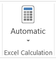
The Excel Calculation icon has the option of Automatic, Automatic Except for Data Tables, and Manual. It is recommended that the Calculation be set to Manual when using OneStream] spreadsheets because the Automatic setting results in an Excel re-calculation every time a OneStream’s interactive workbook changes data (e.g., when navigating a Quick View). However, this is not forced because a user might prefer Excel’s Automatic calculation, especially when there is not a significant amount of OneStream data in the workbook.
Excel Add-In › Add-In Components
The Excel Add-In stores error log details on your local drive in the AppData folder. This allows customers and customer support to retrieve log details when experiencing Excel Add-In related issues, resulting in decreased time to resolution.
Error logs in the folder will automatically be deleted after 60 days.
Excel Add-In
Excel Add-In › Work with Data
Cube View Connection Settings
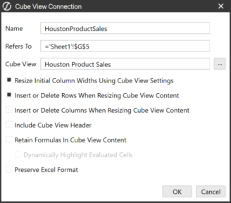
When you create a new Cube View Connection, you can populate the following settings:
| Property | Description |
| Name | The name is created for you if you select the Cube View first. If you type a name first and then select the Cube View, the typed name is retained. |
| Refers To | This setting specifies the starting cell or range in your spreadsheet for the Cube View. It establishes the default cell or range reference for the Cube View Connection. |
| Cube View | Click the ellipsis to look up and add a Cube View to make a Cube View Connection with. |
| Resize Initial Column Widths Using Cube View Settings | Selected by default, this option automatically re-sizes column widths based on the settings from the Cube View selected. |
| Insert or Delete Rows When Resizing Cube View Content | Select this option if you plan to stack everything vertically on your worksheet. This automatically adds or deletes rows as a Cube View expands and contracts. |
| Insert or Delete Columns When Resizing Cube View Content | Select this option if you plan to stack everything horizontally on your worksheet. This automatically adds or deletes columns as a Cube View expands and contracts. |
| Include Cube View Header | This option includes the header on the Cube View. |
| Retain Formulas in Cube View Content | This option allows you to enter formulas in the Cube View (Excel or Spreadsheet) and retain those formulas before and after submission of the sheet or workbook. |
| Dynamically Evaluate Highlighted Cells | This option is only available if the previous option is selected. This highlights a cell if the formula reference has changed without having to refresh a spreadsheet. |
| Preserve Excel Format | This option enables you to preserve native Excel formatting changes made to Cube Views. When enabled, formatting changes made via native Excel formatting will be retained. |
|
Add Parameter Selectors to Sheet |
Selecting this option will generate parameter selectors for all parameters in the selected Cube View, including any dependent parameters. These parameter selectors can be drop-down menus or free-form cell inputs. This option must be selected during the creation process and cannot be added retroactively. To edit parameters added during the creation of a new Cube View Connection, navigate to OneStream > General > Parameters from the Excel or Spreadsheet ribbon. NOTE: If parameters are created using Add Parameter Selectors to Sheet, they will need to be manually deleted from the Parameters ribbon if the associated Cube View Connection is deleted. Deleting the connection alone will orphan the parameters that were added to the sheet. |
Add a Cube View to Excel
Add a Cube View to an Excel sheet using the below steps:
-
Click Cube Views > Cube View Connections.
-
From this window, the cube views added to an Excel workbook can be managed. You can add, remove, edit, or go to styles. Click Add, to add a new Cube View.
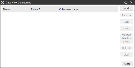
-
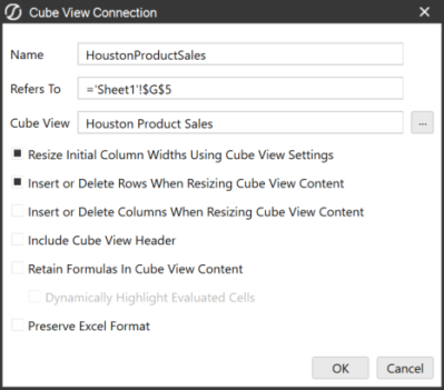
Name the connection and then choose the Cube View.
-
Populate the following fields:
-
Resize Initial Column Widths Using Cube View Settings is the default setting. If you disable it, you can change the columns and save the Cube View. However, if you go back into the same Cube View Connection, the check box will be enabled and you’ll need to disable it again to keep your new cube view settings.
-
Insert or Delete Rows/Colums When Resizing Cube View Content: Select whether there needs to be inserted or deleted rows and/or columns when resizing. This setting will move around other content in the sheets if the size of the Cube View changed since the last refresh.
-
Include Cube View Header: Choose whether to add header rows to the spreadsheet.
-
Retain Formulas in Cube View Content allows you to enter formulas in the Cube View (Excel or Spreadsheet) and retain those formulas pre and post submission of the sheet or workbook. When the sheet or workbook is refreshed the formulas will remain. If the value resulting from the value is different than the value of the OneStream database, the cell will initially become a dirty cell and will turn the cell format to yellow. See Retain Formulas in Cube View Content in Excel and Spreadsheet.
NOTE: When using external Excel workbooks, or after any updates to referenced sheets within the same workbook, you must Refresh Sheet to visualize the dirty cells and then Submit Sheet, unless Dynamically Highlighted Evaluated Cells is turned on.
-
Preserve Excel Format: This option enables you to preserve native Excel formatting changes made to Cube Views. When enabled, formatting changes made via native Excel formatting will be retained. See Preserve Formatting.
-
-
Click the OK button and then the Close button to view your Cube View.
After the Cube View is added, it will appear on the sheet. If formatting was applied to the Cube View, see Cube Views in Presentation, the formatting will come forward into the Excel sheet. Otherwise, apply Excel Styles. These styles are stored in the Excel sheet and can be copied between workbooks. For more information on Excel Styles, see Styles. If you enabled Preserve Excel Format, your formatting will remain. See Preserve Formatting.
NOTE: In order to copy Excel spreadsheet cells into a Data Explorer Grid on the web, click CTRL, select the cells desired, and then click CTRL-C. Navigate to the Data Explorer Grid, select a cell, and click CTRL-V, this will paste the cells into the grid. This can also be done from a Data Explorer Grid into an Excel Spreadsheet.
Retain Formulas in Cube View Content in Excel and Spreadsheet
Retain Formulas in Cube View Content allows you to form Cube View grids of data in Excel, using the Cube Views menu function, that can be linked to other Excel models for easy submission into OneStream. This feature allows formulas, (to writeable cells,) in Excel (or Spreadsheet) for an attached Cube View to be retained on submission and retrieval instead of being replaced with the value of the represented formula.
The Retain Formulas in Cube View Content feature, allows users to plan, budget or forecast and use the familiar functionality of Excel while still submitting data back to the OneStream database.
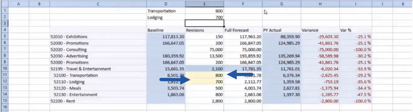
Use the Retain Formulas in Cube View Content feature to enter formulas in the Cube View (Excel or Spreadsheet) and retain those formulas pre and post submission of the sheet or workbook. When the sheet or workbook is refreshed, the formulas will remain. If the value resulting from the formula differs from the existing value in the OneStream database, the cell will initially become a dirty cell and will turn the cell format to yellow.
NOTE: When using external Excel workbooks, or after any updates to referenced sheets within the same workbook, you must Refresh Sheet to visualize the dirty cells and then Submit Sheet, unless you’ve turned on Dynamically Highlight Evaluated Cells in the cube view.
Retain Formulas in Cube View Content links to other Excel worksheets or worksheets in other Excel workbooks.
-
From the OneStream menu, select Cube Views > Cube View Connections.
-
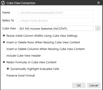
Click Add in the Cube View Connection window or click Edit if you already have a cube view.
-
Click Retain Formulas in Cube View Content box and click the OK button.
-
Add the Cube View, if one is not already selected, and click the Close button.
Dynamically Highlight Evaluated Cells in Excel or Spreadsheet
When Retain Formulas in Cube View Content is enabled, the option to Dynamically Highlight Evaluated Cells becomes available to enable. When it’s enabled, every time you make a change to a cell in Excel or Spreadsheet that is referenced in a Cube View, the cell will immediately update and show the update with a change in color. This cell update is called a dirty cell, which indicates that the cell value is different from the information in the OneStream database.
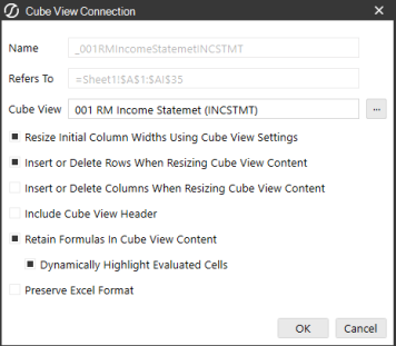
Dynamically Highlight Evaluated Cells saves you a step because the cell changes without requiring a refresh. This feature evaluates all the cells in the spreadsheet and identifies the values in the cube view that have changed relative to its original value in the database.
Excel users who want to continue working in Excel to access can log in through the OneStream menu, update the cube view content and submit it to the database without leaving Excel. You can also perform these tasks in Spreadsheet within the application.
You can Retain Formulas in a Cube View Content that are related to values within a function, existing workbook, sheet, other sheets, in external workbooks, and in external renamed worksheets in Excel. Spreadsheet also offers this functionality, but it doesn’t allow you to point the cell references to external workbooks.
Click Refresh Sheet to see all changes within the cube view content and then click Submit Sheet or activate Dynamically Highlight Evaluated Cells and the cell updates automatically.
The number of cells with formulas in the cube view determines the amount of time it takes to update the cells. You can turn the feature on or off and only use Refresh Sheet to update the values in the cells. Changes will show very quickly, no matter the size of the worksheet, when using Spreadsheet.
Using Retain Formulas and Dynamically Highlight Evaluated Cells
You can also use retain formulas and dynamically highlighted evaluated cells within a cube view to automatically display updated values in an existing workbook, a sheet or sheets, external workbooks, and external renamed worksheets in Excel. You can also do this in Spreadsheet within the OneStream application, however, you can’t point the cell references to external workbooks.
-
In Excel, go to the OneStream menu and Log on.
-
Click Cube Views > Cube View Connections.
-
Click the Add button.
-
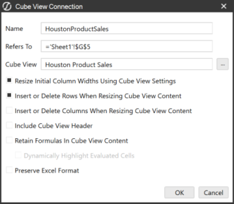
In the Cube View Connection window, click the ellipsis next to the Cube View field.
-
Select your choice and click the OK button.
-
Click Retain Formulas in Cube View Content to activate Dynamically Highlight Evaluated Cells.
-
Then click Dynamically Highlight Evaluated Cells so you can see the changes as they are made.
-
Even if you don’t activate the dynamically highlight evaluated cells feature, you can click Refresh Sheet after you make changes to see them.
-
If you’re prompted, click OK once you’ve selected the parameters for the cube view.
-
Once the cube view has been added, you can click Edit to review, if needed.
-
Make changes to the sheet and press <Enter> to see the updated cell, which will change from white to yellow.
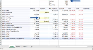
-
Click Submit Sheet to automatically save changes to the database.
Use Cases
These use cases are for both Excel and Spreadsheet unless otherwise noted.
The placing of formulas or cell references. Retain Formulas can reference the following types of formulas. In all instances the formula will stay after refresh and/or submission.
Cell References of individual cells of data on the same sheet.
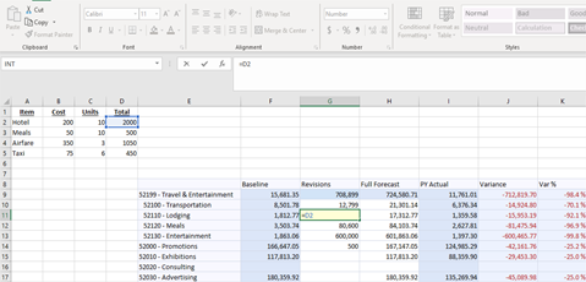
Cell References to a cell on the same sheet, factored by another value.
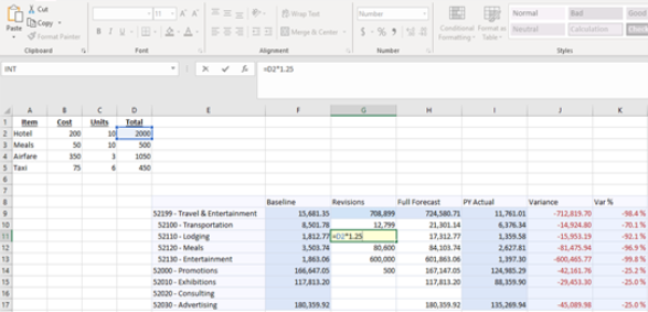
Cell References to cells on other sheets. These can also be factored by another value as well.
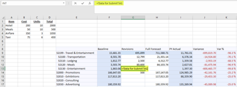
Referenced cell(s) on another saved workbook can also be factored by another value.
NOTE: This applies to Excel only.
Best Practices
Well-Formed Grid
It is suggested to create a “Well-Formed Grid” (Root.List or Comma Separated List) in Cube Views. When using this “Well-Formed Grid” (Root.List or Comma Separated List) in Cube Views, the Excel/SpreadSheet relative (=C2) and absolute formulas (=$C$2) will be retained.
However, when using these relative and absolute formulas within an Excel and Spreadsheet formula, users can use either the cell reference or text within the formula depending upon how members will be added or removed:
-
=VLOOKUP(D30,Sheet1!A:B,2,FALSE) will work in a List or Comma-Separated list (Well-formed grid) when Accounts are added to the end.
-
=VLOOKUP("52000 - Promotions",Sheet1!A:B,2,FALSE) will work in a case when a Member of a Row is moved up or down.
Member Expansion Functions
When using Member Expansion Functions in Cube Views for Excel and SpreadSheet, the cell being referenced within the function (Vlookup, etc), will need to be adjusted and/or referenced as text.
-
=VLOOKUP("52000 - Promotions",Sheet1!A:B,2,FALSE) will work in a Dynamic or when a Member of a Row is moved.
-
=VLOOKUP(D30,Sheet1!A:B,2,FALSE) will NOT work in a Dynamic or when a Member of a Row is moved as this is using the cell ref of D30.
Other Considerations
-
Deselecting the Retain Formulas for Cube View Content will eliminate all formulas that were established /existed on the Cube View grid.
-
Pivoting the existing Dimensions of the Cube View will break formulas.
-
Changing the “structure” of the Cube View grid in the rows or columns will also break the formulas. For example; If you have Account, Entity, UD3 as the dimensions used in the row and switch it to UD3, Entity, Account, it will break the formulas.
-
Users can change the POV to select a new dimension. This will change the Cube View results but retain the existing formulas that were established. The user at this point can choose to utilize the existing formulas, modify or delete. If the original formulas are modified or deleted, the last action will be saved.
-
Linking a white cell (writeable cell) to another cell in a different workbook will work ONLY in Excel and NOT in Spreadsheet.
-
Prior to establishing links to an external workbook, the user should save the external workbook being referenced.
-
When the user renames or saves as the (referenced) file, the user will need to update the links to the newly created file. Updating the links on the spreadsheet should be done BEFORE doing a refresh or submit.
-
Formulas with cell references (VLOOKUP, INDEX(MATCH(, etc) that return errors (#N/A, #ERROR, etc) or non-numeric data will not retain the formula and return to its original value from the Cube View ; this error text cannot be converted into a number so the formulas will not retain.
-
If a Dimension Member Name is renamed; i.e.; “52200 – Rent” is now “52200 – Rent Commercial”, the formula will break.
Excel Add-In › Work with Data › Cube Views
Well-designed Cube Views help you create flexible and rich Excel-based forms and reports. You can retrieve capabilities through formula, but inserting Cube Views in a spreadsheet offers a richer experience with less maintenance.
Named Regions
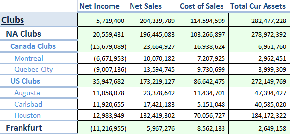
Bringing a Cube View into Excel creates several Named Regions that you can select, refer to, and use with Styles. Named Regions are created for the Cube View, column headers, row headers, and data sections.
If there are multiple named columns or rows in the Cube View, go to the intersection-based Named Regions and use different formatting to differentiate sections. For example, a Total row is separated from detailed data. This combination of Named Regions and Styles generates a nicely formatted report:
Excel Add-In › Work with Data › Cube Views
Cube views are the primary reporting tool in OneStream to display financial data for your organizational needs. You can also use cube view reporting in the Spreadsheet and Excel Add-in using cube view connections.
Define Cube View Connections
Cube view connections are different from exporting a cube view to Excel because the connection remains live, meaning data can be refreshed and submitted.
Before defining cube view connections:
-
Make sure you have the appropriate security settings to access your Cube View and the Spreadsheet page in OneStream.
-
Make sure your cube view is in a group within a profile that has visibility set for Excel.
-
If using the Excel Add-in, connect to OneStream. In Excel, from the OneStream menu, click Logon.
To add a cube view to Excel or Spreadsheet:
-
Select the cell that you want to place the cube view on. The uppermost left corner of your cube view will start on the cell you have selected.
-
Select Cube Views > Cube View Connections > Add from the OneStream ribbon.
Configure Cube View Connections
You can configure cube view connections in OneStream from the Spreadsheet functionality.
-
Click OneStream from the Spreadsheet ribbon.
-
From Cube Views, select Cube View Connections to open the cube view connections dialog box.
Add a Cube View to Excel or Spreadsheet
-
Click Add to create a cube view connection.
-
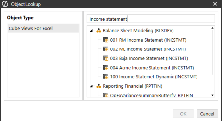
Click the ellipsis next to the Cube View field to open the Object Lookup dialog box. Object Lookup enables you to search for an existing cube view.
-
Use the Filter box to search for the name of the cube view and select it from the list of results.
-
Click the OK button to confirm the cube view selection.
-
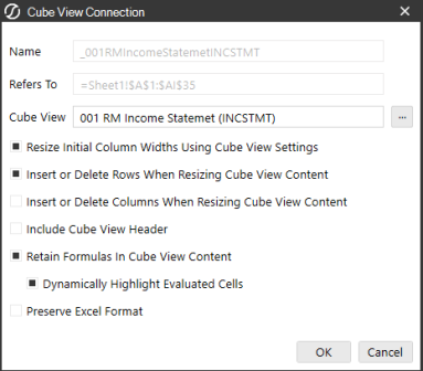
The Name and Refers To fields automatically populate for the selected cube view. Click the OK button to continue.
-
Click Close to exit the dialog box. Your selected cube view is now added to the spreadsheet.
NOTE: See Cube Views for more context on these properties.
Format Cube View Connections
In Spreadsheet, you can apply standard formatting to a cell, a group of cells, or to a row or column. Check the Preserve Excel Formatting setting in the Cube View Connection dialog box, or use Selection Styles and Named Ranges to format a Cube View Connection in Spreadsheet. See Formatting in Excel.
Excel Add-In › Work with Data
Quick views are ad hoc reports that allow you to pivot, drill back, create data sets, and design workbooks to analyze data. Quick views can also be used to submit data. You can create a quick view by:
-
Entering members.
-
Copying and modifying another quick view.
Quick views function similarly to cube views. .
Manage Quick Views
The Quick Views tab displays your dimensions. You can move and replace the default Time and Account dimensions. This table identifies the tasks you can perform on the Quick Views tab.
|
Button |
Description |
|---|---|
|
|
Create a quick view. |
|
|
Rebuild a quick view created by direct data entry by selecting new or modified fields. |
|
|
Rename a quick view. |
|
|
Delete a quick view. |
|
|
Edit quick view properties. |
|
|
Refresh a quick view with the latest data set. |
|
|
Undo up to 100 changes. |
|
|
Restore deleted changes. |
|
|
Select members, identified by dimension type or dimension, to add to a quick view. |
|
|
Clear everything except selected items. |
|
|
Clear only a selected item. |
|
|
Go to the next level in the hierarchy. |
|
|
Go to the top of the hierarchy. |
|
|
Go to the parent member. |
|
|
Go to the immediate child members. |
|
|
Go to the branch base. |


Quick View POV
If you do not select a member, the quick view POV reflects your default POV settings. User-defined descriptions also display in the quick view POV. Hover over dimension labels to view dimension descriptions.
Create and Modify Quick Views
This topic describes how to define and modify quick views.
Create Quick Views
Create a quick view using a sample income statement account. See Find and Add Members to Quick Views and Manage Quick Views.
-
In Cell A2 specify the row: DimensionToken#MemberName A#IncomeStatement.
-
In Cell B1 specify the column: DimensionToken#MemberName T#2018M1.
-
Highlight the dimensions you entered and click Create Quick View. If you are using the Excel Add-in, click the Quick Views tab.

-
In the Create Quick View window, click OK.
You can create quick views using the Quick Views menu on the OneStream ribbon.
-
On the OneStream ribbon, click the Quick Views drop-down menu.
-
Click Create Quick View and one will populate in the cells below.
NOTE: When Preserve Excel Format is enabled on Quick Views, structural changes such as drill down, will not adjust formatting automatically. Manual reformatting may be required when modifying Quick Views.
To add members to your new quick view, manually enter the dimension tokens into the cells or add them using the Quick View toolbar.
-
In cell B1 specify the column: DimensionToken# MemberName S#Actual
-
In cell C1 specify the column: DimensionToken#Member Name S#BudgetV2
-
Click on the cell where your quick view rows will begin. In this example, specify column A2.
-
Click Select Member from the quick view toolbar to the right of the screen.
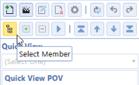
-
From the Select Member dialog box, move dimensions to include in your quick view to the Result List using the single arrow. Click OK.
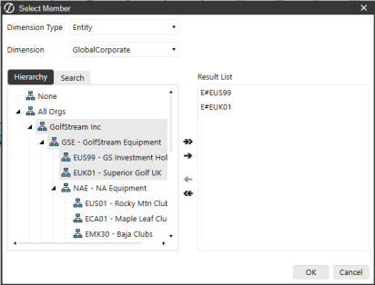
-
Highlight the cells with your data and click Create Quick View.
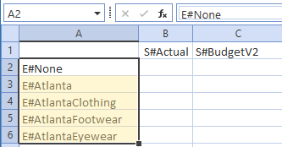
You can create a quick view by copying an existing quick view or expanding on the data in a quick view cell.
-
Select an existing quick view.
-
On the OneStream ribbon, click the Quick Views drop-down menu.
-
Select Copy Quick View.
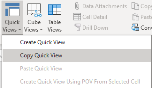
-
Select any cell within the current sheet, workbook, or another workbook.
NOTE: You can only paste a copied Quick View into the same workbook when using Spreadsheet.
-
Click Quick Views drop-down menu and select Paste Quick View.
NOTE: Paste any quick view by right-clicking > Quick View > Paste Quick View. See Right-Click Options.
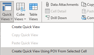
To create a quick view based on the POV from a single cell in an existing quick view:
-
Select an intersection of data in an existing quick view.
-
On the OneStream ribbon, click the Quick Views drop-down menu.
-
Select Create Quick View Using POV From Selected Cell.
Modify Quick Views
The following section outlines how to rebuild quick views after adding or removing dimensions and members.
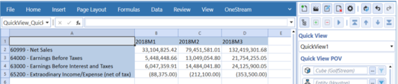
Use a comma-separated member list in column and row cells to build the quick view. In this example, enter:
-
DimensionToken#Root: A#60999,64000,63000,65200 in A2
-
DimensionToken#Root: T#2018M1,2018M2,2018M3 in B1
-
Select the updated area and click Create Quick View.
-
Enter a quick view name and click OK.
The quick view is displayed:
Use the member expansion functions in cells to refine the quick view. For example, enter:
-
DimensionToken#Root A#Root.Children in A2
-
DimensionToken#Root T#2018.Base in B1
-
Select the updated area, click Create Quick View and specify a name.

Use the member expansion functions to enter comma-separated members in cells to finalize the quick view. For example, enter:
-
DimensionToken#Root A#Root.List(60999,64000,63000,65200) in A2
-
DimensionToken#Root T#2018M1 in B1
-
Select the updated area and click Create Quick View.
The quick view updates:

NOTE: Check the suppression options if items do not display as expected.
Extend a Quick View
To add a dimension or new dimension member to a quick view, enter # before the specified dimension or member names. If the dimension is already used, # is not required.
-
Specify the data to use. For example, enter:
Dimension type, such as DimensionToken#MemberName S#Actual
-
Select the area and click Rebuild Quick View.

The updated quick view is displayed:

Change Dimension Members
You can switch dimension members by entering another member name. You do not need to specify a dimension token if you switch to members in a dimension that is being used. For example:
-
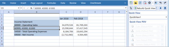
Enter these members: 60999, 43000, and 61000 .
-
Select the members and click Rebuild Quick View.
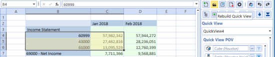
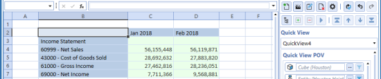
Members 60999, 43000, and 61000 replace 60000 and 54500 as shown in the updated quick view:
You can change from one dimension to another by entering comma-separated members in the same cell. In the example below, the Account dimension is changed to the Entity dimension.
-
Above the Time dimension enter the following, separated by commas:
-
E#HoustonHeights
-
South Houston
-
Operating Sales A#60000

-
-
Select the area and click Rebuild Quick View.
Operating Sales columns are created for the Houston entities:

You can add to an existing dimension's members by entering comma-separated member names in the same cell. If names are numeric or start with an apostrophe, insert a space after each comma.
-
In the same cell, enter the following members. Insert a space after each comma because the member names are numeric.
-
60999
-
43000
-
61000
-
-
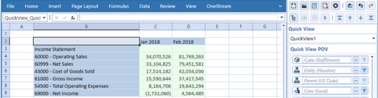
Select the area and click Rebuild Quick View.
Members 60999, 43000, and 61000 are added to the existing member list:
Change Dimensions
Dimensions can be replaced by modifying row and column headers with the updated dimension information and rebuilding the quick view.
-
Click the dimension to be changed, then specify the dimension to use. As shown in the example below, you could:
-
Replace Account with an Entity such as E#HoustonHeights.
-
Add OperatingSales A#60000 above Time.
-
-
Select the area and click Rebuild Quick View.
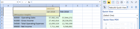
The updated quick view will look like this:

Using "Keep Only" When Extending a Quick View
When modifying a quick view, select the rows and columns you want to remain unchanged using the Keep Only option. This allows you to clear a quick view without losing selected data.
-
In the row below an existing dimension, add these members: 60000, 61000, and 54500.
-
Select the area and click Keep Only.
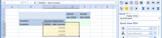
After updating, the quick view will look like this: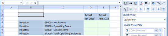
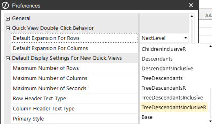
Reverse Member Display Order
You can double-click to reverse the display order of members by specifying Quick View Double-Click preferences.
-
Select Administration > Preferences.
-
In Quick View Double-Click, set Default Expansion for Rows to TreeDescendantsR.
Format and Suppress Data
Use the following to manage and customize your quick view display:
-
Row Header/Columns Header Text Types: Reformat columns and rows.
-
Suppress Repeating Member Names: Display or hide repeating member names. For example, if False, the repeating name displays in each row.
-
Data Style: Apply a provided or custom data style. See Styles.
-
Suppress Invalid Rows/Columns: Hide cells that have invalid data.
-
Zero Suppression Threshold: Suppress all values that are less than a number you specify, for rounding purposes. For example, specifying 499.99 suppresses any value less than that, such as 499.19.
Find and Add Members to Quick Views
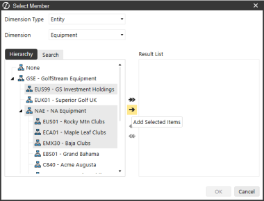
You can add multiple members to a quick view, filtering and searching as necessary.
NOTE: To add members while preserving the current quick view column, select the columns to fill outside the current quick view range. After adding members, select the new column range and click Rebuild Quick View.
-
Select a dimension, then click Select Member.
-
On the Select Members dialog box, perform a task:
-
To find members not shown in the hierarchy, click the Search tab, enter the member name, select members, and then click Add Selected Items.
-
To select multiple members, press Ctrl or Shift, selecting the members, and then click Add Selected Items.
-
-
Select the area to which the members were added and click Rebuild Quick View.
Excel Add-In › Work with Data
A Table View definition for the Windows Application Spreadsheet Tool is defined in a Business Rule. The Administrator designing the rule can define the rows and columns which should be returned to the Spreadsheet from the source table presented in the Table View.
The Table View Business Rule can collect data from multiple data sources. For example, a single Spreadsheet worksheet can display a Table View which collects data from two or more sources.
The Administrator has full control over the write back “save” process through Business Rules. When designing the Table View Business Rule, the BRAPI Authorization functions should be designed into the Business Rule to control access to the viewing or modifying the data. This can be applied to the entire table or to specific cells. A workbook can contain multiple Table Views. These can be on the same worksheet or across worksheet pages.
A single Business Rule file can be used to define multiple Table Views by calling the Business Rule argument, TableViewName. Additionally, a single named range can be used to manage table data cells within the Spreadsheet using user defined named ranges (XFTV_*).
NOTE: When browsing for Table Views Business Rule, only Spreadsheet Type Rules will be displayed in the Object Lookup dialog.
Excel Add-In › Work with Data › Table Views
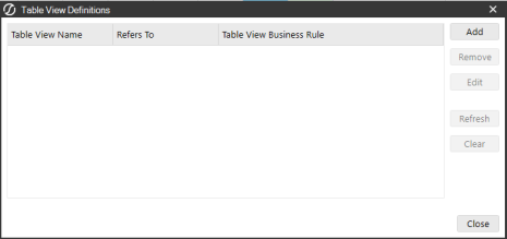
Insert a Table View into Excel.
-
Click Table Views to open the Table View Definition dialog box.
-
From this window, manage the Table Views within Excel. Add, remove, edit, and refresh tables. Click the Add button to add a new Table View.
-
In the Table View Definition dialog box, populate the following fields:
-
Name: Table View name.
-
Refers To: Cell range where the Table View will exist.
-
Table View Business Rule: Click the ellipses to search for and select a business rule.
-
Insert or Delete Rows When Resizing Table View Content: Select this option if you plan to stack everything vertically on your worksheet. This automatically adds or deletes rows as a table view expands and contracts.
-
Insert or Delete Columns When Resizing Table View Content: Select this option if you plan to stack everything horizontally on your worksheet. This automatically adds or deletes columns as a cube view expands and contracts.
-
Preserve Excel Format: This option enables you to preserve native Excel formatting changes made to cube views, quick views, and table views. When enabled, formatting changes made via native Excel formatting will be retained. See Preserve Formatting.
-
-
Click the OK button, then the Close button to view the Table View in the Excel worksheet.
Excel Add-In › Work with Data › Table Views
Table Views is a OneStream Windows Application only spreadsheet control. The primary purpose of Table Views is to provide an easier method to creating Dashboards where relational data is required. The use of Table Views in Spreadsheet enables the designer to work in a more flexible environment to design a form or data collection tool.
Accessed via the OneStream Windows Application Spreadsheet, the Table Views provide a client-based tool to support Dashboard forms. Table Views are not intended as an alternative to other tools, such as the SQL Table Editor or Grid Viewer, Dashboard Components.
Key Use
-
Tool kit item for advanced OneStream Solution or dashboard designers
-
Designed to collect records from relational tables, or other sources
-
Present the information in the Spreadsheet format
-
Utilize client-side functionality, found in the Spreadsheet tool, such as calculations and pick-list validation lists
-
Update table records only
Design Considerations
-
The current functionality is designed to update records in target tables
-
Does not perform inserts, to create new records
-
Controlling elements must be designed into the Table View Business Rule by the creator to ensure data integrity, security and performance
Table View Size Considerations
-
Spreadsheet support of Table Views depends upon the number of rows and row content
-
The Spreadsheet Control does not support paging, therefore all rows and content must be returned
-
Performance testing and design expectations is to support approximately 8000 KB of data per Table View.
Excel Add-In › Work with Data
Generate a drop-down menu in a Cube View or Table View column based on selected parameters in the Excel Add-In or Spreadsheet to quickly filter your data. This functionality eliminates the need to manually create drop-down menus. When a parameter in the drop-down menu is changed, the worksheet will refresh to show the updated output. Parameters that are dependent on one another will updated automatically when the related parameter is altered.
NOTE: See Table View Columns to set up your business rule code to generate a nested parameter in a column in a Table View.
Supported Parameters
The following types of parameters are supported:
-
Literal
-
Input
-
Delimited
-
Bound
-
Member

Unsupported Parameters
The member dialog parameter is not supported.
Create a Parameter
Follow these steps to create a parameter driven drop-down menu for a Cube View:
-
Select the cell to display the drop-down menu.
-
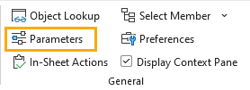
In the Excel ribbon, navigate to OneStream > General > Parameters.
-
In the Parameters dialog box, click the Add button.
-
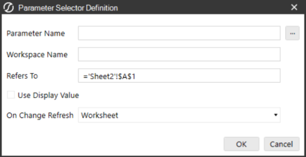
In the Parameter Selector Definition dialog box, populate the following fields:
-
Parameter Name: Click the ellipsis to search for and select the parameter. The name is automatically populated based on the selected parameter.
NOTE: It is best practice when creating parameters that the names be unique, even across Workspaces.
-
Workspace Name: Name of the application workspace of the parameter. This field automatically populates when a parameter is selected.
-
Refers To: Cell or range that will display the button.
-
Use Display Value: The Use Display Value setting enables you to choose which item to use in your drop-down menus. In Application > Workspaces > [...] > Parameters, you can configure Display and Value Items.
For example, if you configure the following settings:
-
Display Items: MI, OH
-
Value Items: Michigan, OH
Then, if Use Display Value is selected, the Display Items (MI and OH) will display in the drop-down menu. If it is clear, the Value Items (Michigan and OH) will display.
-
-
On Change Refresh: When you switch parameters, refresh the worksheet or workbook. Select Nothing to keep the sheet as is.
-
Click the OK button, then click the Close button on the Parameters dialog box.
Parameter Best Practices
-
When working with parameters in Excel and Spreadsheet, remember that nested parameters and input parameters need to be consumed by a Cube View or Table View. Using nested, standalone parameters may generate undesirable results.
-
When adding dependent parameters to a worksheet manually, remember that parameters must be added in the order in which their sequence must be resolved. When using Add Parameter Selectors to Sheet, the parameters will automatically be added in their sequential orde.r
Example: Year must be added before Month. Region must be added before Sub-Region.
-
For dependent parameters to refresh correctly when the parent parameter is changed, the Workspace containing the Cube View or dependent parameter within the Spreadsheet or the Excel Add-In must be sharable. To enable this, navigate to Application > Workspaces > Sharing and ensure Is Sharable Workspace is set to True.
Excel Add-In › Work with Data
In-sheet actions enable you to quickly interact with your data directly in Excel and Spreadsheet. Creating a button streamlines the following actions:
-
Refreshing a worksheet or workbook
-
Submitting a worksheet or workbook
-
Running a data management sequence
Create In-Sheet Button
Build an In-Sheet Action button using these steps:
-
Navigate to the Excel worksheet you would like to place your In-Sheet Action.
-
Select a cell.
NOTE: Make any In-Sheet Action button larger by selecting multiple cells. If a button consists of more than one cell, when opened in Spreadsheet, the button will revert to a single cell.
-
From the ribbon, select OneStream > General > In-Sheet Actions.
-
In the In-Sheet Actions dialog, click the Add button.
-
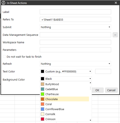
In the next In-Sheet Actions dialog, populate any applicable fields:
-
Label: Button text to show in cell.
-
Refers To: Cell or range where the button will appear.
-
Submit: Submits the Worksheet or Workbook after clicking the button. Select Nothing from the drop-down menu if you do not want to make a submission.
-
Data Management Sequence: Use your In-Sheet action button to run a data management job. Click the ellipsis to browse for and select a data management sequence.
-
Workspace Name: Populates with the name of the Workspace after you select a data management sequence.
-
Parameters: Designate explicit values for parameters needed for your data management sequence or leave blank to resolve parameters based on sheet selections. Enter the parameter name and the value it should be set to at run time, for example, myparam = value. When adding multiple parameters, separate each parameter with a comma. For example, myparam=value1, myparam2=value2. If the value for your parameter contains a space, use brackets in your syntax. For example, myparam=[South Houston].
IMPORTANT: Parameters can only be used if they have been resolved in an existing Cube View or Table View in the sheet or workbook. To use parameters that don't exist in your Cube View or Table View, add it anywhere in the Cube View in OneStream, for example in the page caption field or other unused field that does not impact Cube View rendering. For Table Views, add the parameter to the GetCustomSubsVars section of the Spreadsheet business rule.
NOTE: In-sheet actions will not prompt for unresolved parameters.
-
Do not wait for task to finish: Enable this setting to continue working while the data management sequence runs in the background.
-
Refresh: Refreshes the Worksheet or Workbook after clicking the button. Select Nothing from the drop-down menu if you do not want to make a submission.
-
Text Color: Choose a custom button text color and input an eight character hex code, or select a color from the drop-down menu.
-
Background color: Choose a custom button background color and input an eight character hex code, or select a color from the drop-down menu.
-
-
Click the OK button and then the Close button. Your button will appear in the cells you selected.
Format In-Sheet Actions
By default, In-Sheet Action buttons will display as black with white text. After initial creation, customize the display of your buttons by formatting them with custom colors and styles. Modify your button using the steps below:
-
From the ribbon, select OneStream > General > In-Sheet Actions.
-
In the In-Sheet Actions dialog box, select the button to format and click the Edit button.
-
Use the Button Theme drop-down menu to select a color.
-
Click OK and then Close to save changes.
Excel Add-In › Work with Data
When working with data in the in Excel Add-In, right-click and navigate to OneStream to see the following available actions:
Cube Views
Cube View Connections
Create a new Cube View connection.
Selection Styles
Set up a selection style. See Selection Styles.
Manage Selection Styles
Modify an existing selection style. See Selection Styles.
Quick View
For a complete overview on Quick Views, see Quick Views.
Create Quick View
This will create a new Quick View in the worksheet’s selected cell.
Copy Quick View
This will copy the selected Quick View in order to paste a version of it in another spreadsheet or workbook.
Paste Quick View
This will paste the copied quick view to the current spreadsheet or another workbook.P
Create Quick View Using POV from Selected Cell
This will create a new Quick View based on the current POV from the selected cell. This can be done using a Quick View cell’s POV, a Cube View cell’s POV, or a XFGetCell's POV.
Expand
Select the cell of a Member and choose how to view its data. Select from these options:
-
AllTops: This returns the Top of the given Dimension.
-
AllBase
This returns all Base Members of the given Dimension regardless of what Member is selected. -
All
This returns all Members in a given Dimension. -
NextLevel
This returns the next level of Members under the selected Member. -
KeepOnly
This will only keep the selected Members. -
Parents
This returns the direct Parents of the selected Member regardless of how many hierarchies to which the Member belongs. -
Ancestors
This returns all Members up the chain from the selected Member. -
Children
This returns the first level of Children under the selected Member. -
ChildrenInclusive
This returns the selected Member and its first level of Children. -
Descendants
This returns every Member under the selected Member in a list, not a hierarchy. -
DescendantsInclusive
This returns the selected Member and every Member under it in a list, not a hierarchy. -
TreeDescendants
This returns every Member under the selected Member in a hierarchy. -
TreeDescendantsInclusive
This returns the selected Member and every Member under it in a hierarchy. -
Base
This returns the Base level for the selected Member.
Paste POV
Enables you to Paste a POV into a selected cell in order to change the data within that Quick View.
Apply POV from Selected Cell
This enables a POV to be passed from a selected cell within a Quick View.
Apply User POV
This enables a Point of View to be passed between Quick Views.
Clear POV
This clears the POV for the selected Quick View.
For the following properties, see Manage Quick Views
-
Undo
-
Redo
-
Options
-
Refresh
General OneStream Right-Click Options
Calculate, Translate, Consolidate
If permitted, these calculations can be performed on the selected cell. These function the same as the icons in the Ribbon, but you have the choice to do Force operations and additional Logging.
Select Member
Select a Dimension Type from the drop down list in order to view the Members of that Dimension. Select a Member of the hierarchy, and the Member name will display in the selected cell.
Copy POV from Data Cell
This captures the Point of View of the currently selected cell. After clicking this option, the Paste POV As XFGetCell becomes available.
Paste POV as XFGetCell
This option is only available after clicking Copy POV From Data Cell. After clicking this option, OneStream converts the copied cell into an XFGetCell formula.
Convert to XFGetCells
This converts an existing Quick View into an XFGetCells.
Allocate
Data Attachments
This opens the Data Attachments dialog so you can view existing comments or attachments on the selected cell, or to edit data attachments.
Cell Detail
Cell POV Information
This gives a detailed summary of the selected Members related to this intersection as well as the full Member Script used to get this value. All the major properties of these Members can be seen from this dialog.
Cell Status
This returns a long list of properties about a given cell.
Navigate
Enables you to launch a cube view or dashboard from Excel when configured.
Drill Down
Spreading
This enables users to enter data into an aggregate Member, like an annual time period, and spread values over several columns or rows without having to type in each cell’s values. Select from the following options:
-
Spread Selected Cells: See Spreading Types.
-
Flag Selected Cells: Flags selected cells so the original amount in the cell is retained during the spreading process.
-
Clear Flags: Select this to clear any flagged cells.
Excel Add-In › Work with Data
Retrieving and changing data can be done by using functions. To see the functions and their Parameters, open Excel and select the Formulas tab. Select Insert Function and select OneStreamExcelAddIn.XFFunctions where it says to Select a category.
The output of the function will look something like this: =XFGetCell(A1,A2,A3,A4,A5)
The equivalent functions like XFGetCell provide a separate Parameter to specify each Dimension Member without using the Member Script syntax. (e.g., E#CT:A#Sales would not be used, CT and Sales would be used in the correct Parameter for that Dimension)
Here are the main functions to use:
NOTE: If a field within the function is not needed, enter a double quote to ignore it.
XFGetCell
This function retrieves data based on the Parameters supplied. Each Parameter needs to be defined.
Example:
XFGetCell(NoDataAs Zero, Cube, Entity, Parent, Cons, Scenario, Time, View, Account, Flow, Origin, IC, UD1, UD2, UD3, UD4, UD5, UD6, UD7, UD8)
XFGetCell5
This has the same functionality as XFGetCell except it limits the User Defined Dimensions to five instead of eight.
XFGetFXRate
This function retrieves rates from the system. Each Parameter needs to be defined.
XFGetFXRate(DisplayNoDataAsZero, FXRateType, Time, SourceCurrency, DestCurrency)
XFGetCalculatedFxRate
This function directly retrieves an exchange rate even if only the inverse rate exists in the system.
XFGetMemberProperty
This function retrieves any Dimension Member property from the Member Properties tab in the Dimension Library. Note there are no spaces used when defining property name.
Example:
XFGetMemberProperty(“DimTypeName”,“MemberName or Script”,“PropertyName”, “VaryByCubeTypeName”,“VaryByScenarioTypeName”,“VaryByTimeName”)
NOTE: If the function does not need to vary by Cube Type, Scenario, or Time, enter a double quote in order to ignore it.
Example: Retrieving Currency for the Houston Entity
XFGetMemberProperty(“Entity”,”Houston”,”Currency”,””,””,””)
Example: Retrieving an Account Formula that only occurs in the Budget Scenario
XFGetMemberProperty(“Account”,”51000”,”Formula”,””,”Budget”,””)
Example: Retrieving the Short Description Property for Time Dimension
XFGetMemberProperty("Time","2015M8","ShortDescription","","","")
XFGetRelationshipProperty
This function retrieves any Dimension relationship property from the Relationship Properties tab in the Dimension Library.
XFGetRelationshipProperty(“DimTypeName”,“ParentMemberName or Script”,“ChildMemberName or Script”,“PropertyName”,“VaryByScenarioTypeName”,“VaryByTimeName”)
NOTE: If the function does not need to vary by Cube, Scenario, or Time, enter a double quote in order to ignore it.
Example: Retrieving a Flow Members Aggregation Weight
XFGetRelationshipProperty(“Flow”,”TotalBalance”,”Total Movement”,”AggregationWeight”,””,””)
Example: Retrieving an Entity’s Percent Consolidation for July, 2015
XFGetRelationshipProperty(“Entity”,”Houston”,”South Houston”,”PercentConsolidation”,””,”2015M7”)
XFGetHierarchyProperty
This function determines whether or not a Dimension has children and returns True or False.
Example:
XFGetHierarchyProperty(“DimTypeName”,”DimName”,“MemberName or Script”,“PropertyName”,”PrimaryCubeName”,”ScenarioTypeNameForMembers”,”MergeMembersfromReferencedCubes”)
Example: Retrieving Child Hierarchy
XFGetHierarchyProperty("entity","HoustonEntities","Houston Heights","HasChildren","Houston","Actual",FALSE)
XFGetDashboardParameterValue
This function is available to Excel Add-in and Spreadsheet. If that function is used within an XLSX file that is using a function like XFGetCell or XFSetCell (or similar) where these are referencing a custom parameter value (e.g. ParamEntity) that is on the Dashboard that references this Spreadsheet from within it as a Component. The practice to get this Custom Parameter value is to use XFGetDashboardParameterValue to fetch the text from that Parameter or its default value and place it in a cell on the Spreadsheet (e.g. B1). Then the cell that is using a retrieve function such as XFGetCell would reference this other cell (i.e. B1).
XFGetDashboardParameterValue("myParamName", "Text For Default Value")
XFGetMemberInfo
This function retrieves the description in the system. Each Parameter needs to be defined.
XFGetMemberInfo(MemberInfoType, DimTypeName, MemberName, NameorDesc, NameandDesc)
XFInternalGetDataFromServer
This function returns True or False. It does not take any arguments.
XFSetCell
This function saves data to the amount field based on the Parameters supplied. Each Parameter needs to be defined.
XFSetCell(CellValue, StoreZeroAsNoData, Cube, Entity, Parent, Cons, Scenario, Time, View, Account, Flow, Origin, IC, UD1, UD2, UD3, UD4, UD5, UD6, UD7, UD8
XFSetFXRate
This function saves rates to the system. Each Parameter needs to be defined.
XFSetFXRate(Value, StoreZeroAsNoData, FXRateType, Time, SourceCurrency,DestinationCurrency)
XFGetCellUsingScript
XFGetMemberInfoUsingScript
XFSetCellUsingScript
All of the functions that have UsingScript are based on a Member Script (e.g., A#Sales:E#Texas). The multiple Parameters provide the ability to specify multiple portions of the full Member Script using different Excel cells. All of the Member Scripts in the function Parameters combine to create one Member Script. It will then use the combined Member Script to retrieve the data cell.
Example:=XFGetCellUsingScript
(TRUE,"GolfStream","E#Frankfurt:C#Local:S#Actual:T#2022M1:V#YTD:A#10100:F#None:O#Top:I#Top:U1#Top:U2#Top:U3#Top: U4#Top:U5#None:U6#None:U7#None:U8#None","","")
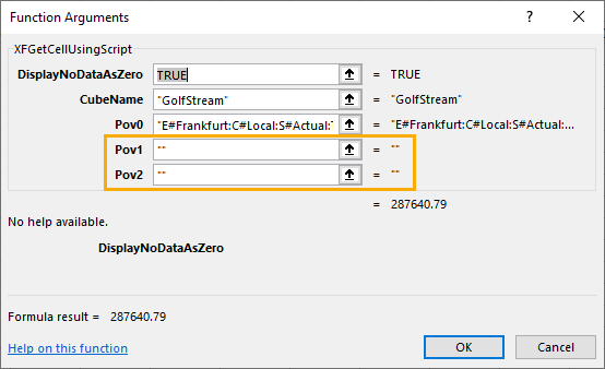
NOTE: Add quotation marks to POVs not being used.
The following examples detail uses of XFGetCellUsingScript.
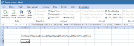
Example:
=XFGetCellUsingScript(TRUE,"GolfStream", "E#[Houston Heights]:C#Local:F#None:S#Actual:T#2017Q2:V#YTD:A#69000:"&D3,"","")
D3= “U6#None:U7#None:U8#None:O#Top:I#Top:U1#Top:U2#Top:U3#Top:U4#Top:U5#None”
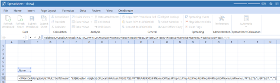
Example:
=XFGetCellUsingScript(TRUE,"GolfStream", "E#[Houston Heights]:C#Local:S#Actual:T#2017Q2:V#YTD:A#69000:F#None:O#Top:I#Top:U1#Top: U2#Top:U3#Top:U4#Top:U5#None:U6#None:U7#"&B7&":U8#"&B7,"","")
B7=”None”
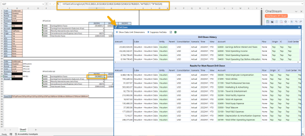
Example:
=XFGetCellUsingScript(TRUE,$B$21,$C$22&$C$23&$C$24&$C$25&$C$27&$B$35,"A#"&$E27,"T#"&G$26)
XFGetCellUsingScriptEx
XFGetMemberInfoUsingScriptEx
XFSetCellUsingScriptEx
All of the functions that have …Ex have many more Parameters to use for combining Member Scripts (e.g., commonly used when creating another version of a function that has extra Parameters). Ex would also be used to combine many Member Script Parameters.
XFSetCellLocalForms
XFGetCellLocalAdjInput5
XFGetCellLocalForms5
XFGetCellLocalImport5
XFGetCellLocalOTop5
XFGetCellTransAdjInput5
XFGetCellTranForms5
XFGetCellTransImport5
XFGetCellTransOTop5
XFSetCellLocalForms5
These functions use the Consolidation and Origin Dimensions. For example, XFSetCellLocalForms is using Local Consolidation and the Forms Origin Member. The number five at the end of the functions limit the User Defined Dimensions to five instead of eight.
XFGetCellUSingScriptVolatile
XFGetCellVolatile
XFGetFXRateVolatile
XFGetMemberInfoUsingScriptExVolatile
XFGetMemberInfoUsingScriptVolatile
XFGetMemberInfoVolatile
XFSetCellUsingScriptExVolatile
XFSetCellUsingScriptVolatile
XFSetCellVolatile
XFSetFXRateVolatile
In some cases, Excel requires a volatile function for proper refreshing, for example, some Excel Charts that reference calculated cells.
XFInternalPrepareCalculationStep
XFInternalSendDatatoServer
XFInternaSetConnectionInfo
All of the functions that begin with XFInternal only work for internal processes.
Excel Add-In › Work with Data
In an existing quick view, you can convert to formula-based retrieves (XFGetCell) on intersections of data using the Convert To XFGetCells option in the top ribbon toolbar.
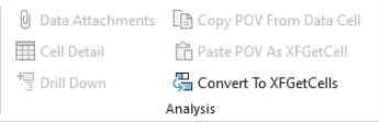
After selecting Convert To XFGetCells, OneStream displays the following prompts:
-
Are you sure you want to convert all the data in Quick View ‘Name of the Quick View’ to XFGetCells?
-
By clicking OK, the Quick View definition will be deleted and specific intersections of data will be converted to XFGetCell formulas.
This is a great way to set up a lot of formulas at once. However, these will hardcode all the dimension members in your formulas. If the member name is being displayed, the rows and columns can be synchronized to the pre-made quick view and cube view rows and columns. Your quick view can be adjusted to display the member name instead of the description through the quick view options.
NOTE: Quick view data that has been converted to XFGetCell cannot be converted back into a quick view. However, quick view content may be saved as a template before converting.
Additionally, XF Functions can be manually entered:
-
Select a cell and click on the insert function icon.
-
Select an XFGet function from the pop-up menu.
-
Fill out the necessary dimensions to build your XF Retrieve. If you do not want to fill one out, place a “” in the property and it defaults to the data in your cube POV.
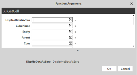
-
Click OK to save the dimensions entered and the selected cell data changes to #REFRESH.
- If your query is in the correct syntax, data populates in the cell after refreshing the sheet.
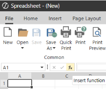
NOTE: If a member name has been misspelled, the cell returns an error calling out the first misspelled member name.
Absolute Cell References
Absolute cell references are a functionality in the Excel Add-in that allows an exact cell reference to be kept when you copy the formula to another cell. To do this, put a $ in front of the portion of the cell reference that you want to keep.
For example, if you want to keep the entire A1 cell reference to copy to another cell you would change the cell reference to $A$1. If you only want to keep the column, the cell reference would be $A1 and if you only want to keep the row it would be A$1.
Relative Cell References
Relative cell references are the default state of cells in an Excel workbook. The reference is relative to the location of the cell. Formulas copied to new cells retain the location information and apply it to the new set of cells.
For example, if you reference A1 in cell C1 and then copy the formula into D1, the results will be a reference to B1 in cell D1 because the formula is referencing 2 columns before.
Excel Add-In › Work with Data
A Sub procedure is a series of Visual Basic statements that perform a specific task. It can take arguments, such as constants, variables, or expressions that are passed by a calling the procedure. If a Sub procedure has no arguments, the Sub statement must include an empty set of parentheses.
A Sub procedure begins with a Sub statement, followed by the tasks to be performed, and ends with an End Sub statement. The following snippet of VBA code represents the structure of a Sub procedure:
Sub [ProcedureName] (Arguments)
[Statements]
End Sub
OneStream Functions are used with Sub procedures to automate data submission from XFSetCells formulas.
NOTE: To use these functions in Excel, you must have the latest version of OneStream and its corresponding Excel add-in installed.
Procedures currently supported are:
-
LogonAndOpenApplication - Login varies depending on the authentication type setup for your application:
NOTE: Resource Owner Password Credentials (ROPC) is no longer supported. As a result, the following ProcessSSOAuthenticationAndCreateToken has been deprecated. See Legacy Single Sign On (SSO) for Bearer Token procedure.
Sub SSOLogon()
Set xfAddIn = Application.COMAddIns("OneStreamExcelAddIn")
If Not xfAddIn Is Nothing Then
If Not xfAddIn.Object Is Nothing Then
ssoToken = xfAddIn.Object.ProcessSSOAuthenticationAndCreateToken
("https://golfstream.onestreamtest.com/OneStreamWeb",
"[email protected]", "P@$$w0&D")
xfUserName = xfAddIn.Object.GetXFUserNameFromSSOToken(ssoToken)-
OneStream IdentityServer (OIS) - (url, PAT, application)
Supports the use of Personal Access Tokens. Refer to the Identity and Access Management Guide for creating and managing PATS.Sub OIS_PAT_Logon()
Set xfAddIn = Application.COMAddIns("OneStreamExcelAddIn")
If Not xfAddIn Is Nothing Then
If Not xfAddIn.Object Is Nothing Then
' OIS using PAT
loggedIn = xfAddIn.Object.LogonAndOpenApplicationWithToken("https://yoursite.onestreamcloud.com/OneStreamWeb", InsertPersonalAccessToken, "GolfStreamDemo_v36")
MsgBox ("Is Logged In : " & loggedIn)
End If
End If
End Sub -
Legacy Single Sign On (SSO) - (url, ssoToken, application)
Supports the use of Bearer token from your identity providerSub SSOLogon()
Set xfAddIn = Application.COMAddIns("OneStreamExcelAddIn")
If Not xfAddIn Is Nothing Then
If Not xfAddIn.Object Is Nothing Then
' Legacy SSO via Bearer Token
Dim ssoToken As String
ssoToken = <obtain Bearer token from your Identity Provider>"
loggedIn = xfAddIn.Object.LogonAndOpenApplicationWithToken("https://yoursite.onestreamcloud.com/OneStreamWeb", ssoToken, "GolfStreamDemo_v36")
MsgBox ("Is Logged In : " & loggedIn)
End If
End If
End Sub -
Native Authentication (Self-hosted) - (url, user, password, application)
Support login via userid and passwordSub Native_Logon()
Set xfAddIn = Application.COMAddIns("OneStreamExcelAddIn")
If Not xfAddIn Is Nothing Then
If Not xfAddIn.Object Is Nothing Then
' Native - UserName & Password
loggedIn = xfAddIn.Object.LogonAndOpenApplication("https://yoursite.onestreamcloud.com/OneStreamWeb", UserName, Password, "GolfStreamDemo_v36")
MsgBox ("Is Logged In ): " & loggedIn)
End If
End If
End Sub
-
-
Logoff()
-
RefreshXFFunctions() -- refer to the following example:
Sub RefreshXFFunctions()
Set xfAddIn = Application.COMAddIns("OneStreamExcelAddIn")
If Not xfAddIn Is Nothing Then
If Not xfAddIn.Object Is Nothing Then
Call xfAddIn.Object.RefreshXFFunctions
End If
End If
End Sub -
RefreshXFFunctionsForActiveWorksheet()
-
RefreshQuickViews()
-
RefreshQuickViewsForActiveWorksheet()
-
RefreshCubeViews()
-
RefreshCubeViewsForActiveWorkSheet()
-
ShowParametersDlg()
-
ShowParametersDlgForActiveWorksheet()
-
SubmitXFFunctions () -- Automates the data loading process and eliminates the need to open the Excel files individually and submit data manually. Using a VBA routine, files with XFSET functions that are linked to other cells, sheets, and files can be programmatically submitted to OneStream. This procedure calls only XFSetCells. Refer to the following example:
Sub SubmitXFFunctionsTest()
 Set xfAddin = Application.COMAddIns("OneStreamExcelAddin")
 If Not xfAddin Is Nothing Then
 If Not xfAddin.Object Is Nothing Then
 Call xfAddin.Object.SubmitXFFunctions
 Call xfAddin.Object.RefreshXFFunctions
 End If
 End If
End Sub
Excel Add-In
These formatting options are available in Excel:
-
Preserve Formatting: Quickly preserve native Excel formatting in Cube Views, Quick Views, and Table Views when you submit or refresh your worksheet.
-
Styles: Create custom styles to consistently format elements, like cells and headings.
-
Conditional: Set styles for conditional text and data within your Excel worksheet.
-
Selection Styles for Cube Views: Bring a Cube View into Excel, and format it using native Excel formatting.
Excel Add-In › Formatting in Excel
When you build a Cube View, Quick View, or Table View you have the option to enable the Preserve Excel Format setting. This setting enables you to preserve local Excel formatting without the need to create custom, conditional, or selection styles. When enabling preserve formatting on Cube Views or Table Views, we recommend disabling the Insert or delete rows or columns when resizing cube view content.
NOTE: When Preserve Excel Format is enabled for Table Views, the DataType column must be specified as numeric.
Enable Preserve Excel Format
To turn on the Preserve Excel Format setting, create a Quick View, Cube View, or Table View. In the respective dialog box, enable the Preserve Excel Format setting.
| Cube View |
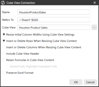
|
| Quick View |
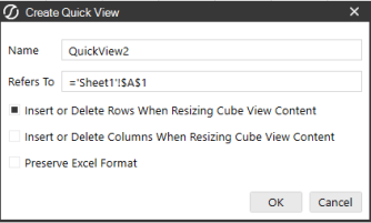
|
|
Table View |
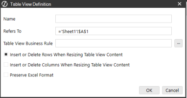
|
On already created views, you can edit the view and enable the setting.
When enabled, changes made to the sheet will be kept, even after you save and refresh your sheet. Additionally, you can copy your view and associated formatting will remain on the duplicated view when the Preserve Excel Format setting is enabled on the source Cube View, Quick View, or Table View.
NOTE: When Preserve Excel Format is enabled on Quick Views, structural changes such as drill down, will not adjust formatting automatically. Manual reformatting may be required when modifying Quick Views.
Excel Add-In › Formatting in Excel
The same standard Styles are used in Excel, however, if you want to create a new style in order to change the format of how the numbers are displayed, see the example that follows.
Creating a Custom Style
The following example was created in the Excel 2010 Version.
On the Home Tab, click on the new style sheet.

Select New Cell Style.
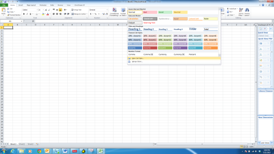
A new style window will appear, click Format.
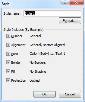
The format page will then display, click Custom.
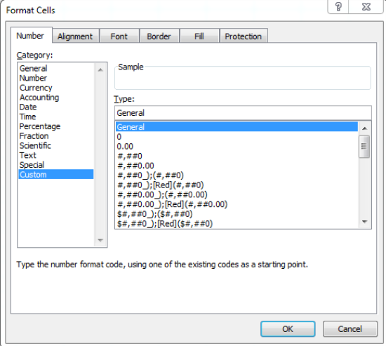
Finally, under Type, enter the custom formatting. This example will be formatting for Millions. (#,,)
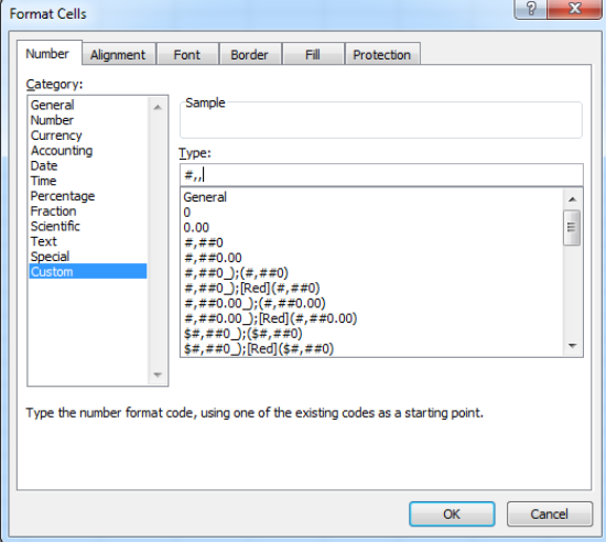
Click OK.
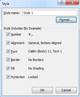
Type in a Style Name and click OK.
Now that a new style sheet has been created in Excel, it can be assigned to a Quick view.
This is the Quick View before the formatting:

To add the formatting, click on the Edit Quick View Options  in the Quick View Tab on the right side of the screen.
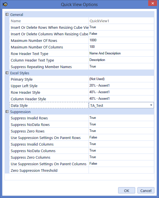
This is the Quick View after the update:

Excel Add-In › Formatting in Excel
Use Conditional Formatting in Cube Views to visually explore and analyze data. You can highlight cells or ranges of cells, identify key values, and represent data using data bars, color scales, and icon sets that correspond to specific variations in the data. If there are any existing formats prior to applying Conditional Formatting, they will be retained if the range of cells containing the conditional formats do not meet the conditions of the rule. All styles from the cube view and the selection styles that had been previously applied to that range are overridden by conditional formatting.
Create Conditional Formatting in an Existing or New Cube View
-
Click Home > Conditional Formatting > Highlight Cells Rules > Greater Than.
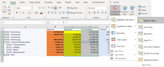
-
Enter 6000 and click OK.
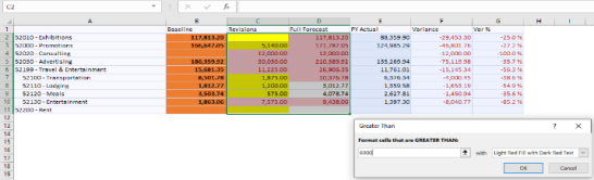
-
Go to OneStream and click Refresh Sheet to see that your changes have been applied.
-
If you make a change that is different than the value in the database, the cell will change to pale yellow, until you refresh or submit.
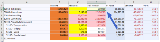
-
If you submit, it will revert to the formatting that was in the cube view since it is no longer greater than 6000.
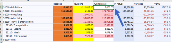
-
If you make a change to a cell that has conditional formatting and a selection style,
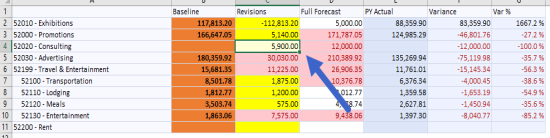
when you submit, it will convert back to the selection style since it is no longer greater than 6000.
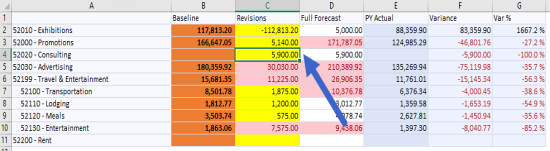
-
To add icons, go Home > Conditional Formatting > Icon Sets and select the icons to use, in this example, select the arrows.
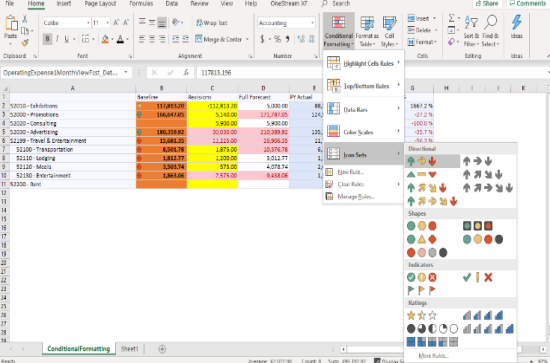
-
The icons are part of the cube view.
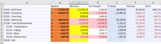
-
You can also create, edit, delete, and view all conditional formatting rules.
-
If you save the workbook, the conditional formatting is saved.
Excel Add-In › Formatting in Excel
Using Selection Styles
You can bring an existing cube view into Excel or Spreadsheet and format using functionality that is included in Excel, to create highly formatted reporting. You can also modify it locally as well as in spreadsheet. You can use existing cube view formatting, add new styles to apply changes to rows, columns, or cells, or a combination of existing styles with new styles, and add conditional formatting.
Creating a Selection Style
-
Log in using the OneStream menu.
-
Click Cube Views > Cube View Connections.
-
Click the Add button.
-
Select the cube view, click the OK button, then the Closebutton.
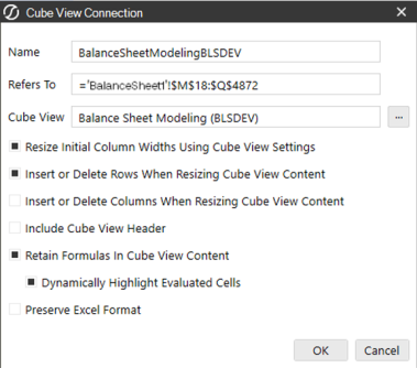
-
Select the cell, a group of cells, a column, or row to format.
.
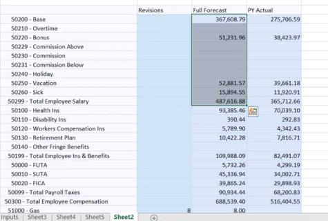
-
Right-click to open Format Cells or use the Home menu to choose formatting.
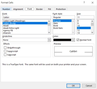
-
After formatting, click OneStream > Cube Views > Selection Styles.
-
Enter a Name and Range to apply to the current Selection, Entire Row, or Entire Column. Then click OK.
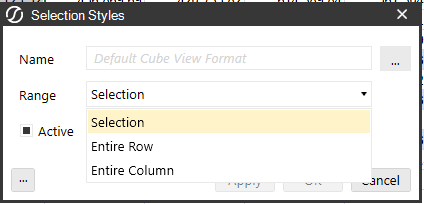
-
The formatting is applied to cube view.
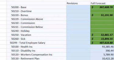
-
Save the file to save the formatting to the cube view.
Using an Existing Style
-
Select the cell, a group of cells, a column, or row to format, then click Cube Views > Selection Styles.
-
Click Excel Styles to select a style. If a style is not selected the Default Cube View Format is used.
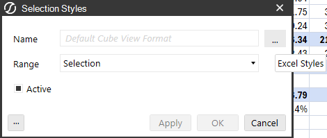
-
On the style palette, hover to view the styles.
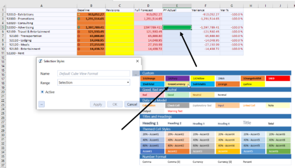
-
Click the style to use and then Apply or OK.
-
Save the file to save the cube view formatting.
Adding a Selection Styles Shortcut
In Excel, right-click Selection Styles then click Add to Quick Access Toolbar. This adds a shortcut to your toolbar that launches the Selection Styles window.

Reviewing Styles and Ranges
-
Click Cube Views > Manage Selection Styles.
-
Review your styles that are applied to the cube view.
-
Modify selected styles.
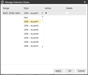
-
Enable or disable Active styles as needed and click OK.
-
Click Apply to preview the changes, or OK to apply the changes.
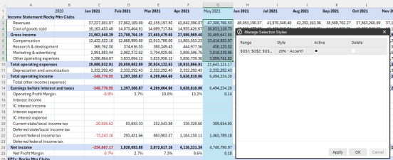
-
In Selection Styles, you will see styles that are no longer Active. Click Activate to enable them.
-
You can delete a style from the cube view but it will be available in the current workbook.
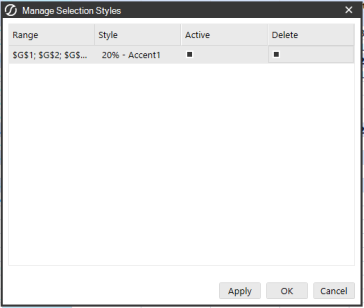
-
Save the file to save the cube view formatting.
Using Right-click Menu Options
You can manage selection styles by right-clicking in a cube view and selecting OneStream > Cube Views > Cube View Connections > Selection Styles > Manage Selection Styles.
Modifying and Duplicate Styles
-
In the Home menu, click Styles and right-click a style.
-
Click Modify or Duplicate and then Format.
-
Make any necessary changes and click OK.
-
Save the file.
Merging Styles
You can use styles created in other workbooks in Excel only.
-
Open a new workbook.
-
Add a cube view.
-
Click Home > Styles then the More arrow.

-
Click Merge Styles, select the style, and click OK.
The style is now available in the workbook.